This paper, addressed by The Shift Project VP Michel Lepetit[1] to Esther L. George (President and CEO of the Federal Reserve Bank of Kansas City, Texas) and Robert S. Kaplan (President and CEO of the Federal Reserve Bank of Dallas), questions the assumptions behind monetary policy’s so called ‘neutrality’.

In the wake of the 2008 Great Financial Crisis the Federal Reserve unleashed a never seen before monetary policy in an attempt to revive the sputtering American economy: Quantitative Easing. This monetary policy took place at a time when world conventional crude oil production had reached its geophysical apex. Instead of looking for low carbon solutions, investors were attracted by riskier investments and greatly contributed to the development of the shale oil industry. Hence, the massive investments in the shale oil industry that followed Quantitative Easing questions the neutrality of monetary policy with regard to the energy industry. If national and international financial institutions were able to skew the global energy production towards more fossil fuel, may it be able to skew it backwards?

Could U.S. Federal Reserve’s recent adhesion to the Network for Green Financial System (NGFS) be seen as a first step on the path towards low-carbon investments?

22^nd of November, 2020 Paris

Is monetary policy (carbon) neutral ?

Dear Mrs. George, Dear Mr. Kaplan,

Thank you for organizing this inspiring virtual conference Navigating the changing Energy Landscape hosted by the Federal Reserve Banks of Dallas and of Kansas City on Friday November 20^th, 2020.

As a finance, energy history and oil macroeconomics specialist, I particularly enjoyed the guest speakers’ provocative thoughts. I highly value their reflexion on the “shale oil revolution” that transformed the Oil & Gas (O&G) industry, and beyond this industry, the world since 2008.

Monetary policy is neutral

The two regions represented at this event account for most of the U.S. oil production surge since 2008 – mostly “unconventional” LTO oil (Light Tight Oil, another name for “shale oil”).

As the head of the Federal Reserve Bank of Dallas, and in unison with many central bankers, Mr Kaplan, you asserted that monetary policy was “neutral”, and that monetary policy tools could not be targeted at particular sectors of the economy[2]. This observation was also mentioned by Mrs George, head of the Federal Reserve Bank of Kansas City, in a thoughtful speech on energy and monetary policy[3]. But since the Federal Reserve (Fed) triggered its extraordinary monetary policy instruments in the 2010s, the macroeconomic mechanisms you both evoked could no longer be effective. In the aftermath of the 2008 Great Financial Crisis, the Fed unleashed a so-called “Unconventional Monetary Policy”: Quantitative Easing (QE).

Speaking of will and intent, the Fed was neutral. Indeed, the Fed’s detailed committee reports of 2009 and 2010 show that it had no intent to develop the U.S. shale oil production, a segment of the oil industry quite marginal at that time[4].

Unconventional Monetary Policy and Unconventional Oil (UMPUO)

Now, if you consider Figure N°1 you will see the quarterly U.S. Oil & Gas CAPEX (O&G CAPEX) at annual rates[5] (in orange; in $Billion (G$); RHS). The figure displays the price of oil (in black; in $ per barrel; same scale: RHS), which is the most well-known driver of O&G CAPEX. The figure also shows the size of the Fed’s balance sheet (in green; in $Billion; LHS) with the timing of the different rounds of Quantitative Easing orchestrated by the Fed. The narrative of the 21^st century world macroeconomic and energetic history (Lepetit 2020) [6] shows how the shale revolution unfolded with the tempo of QE N°1, QE N°2 and QE N°3. From less than $1,000 Billion at the start of 2008, the Fed’s balance sheet reached the impressive amount of $4,500 Billion by the end of 2015.

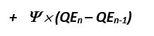
Considering these series and this narrative, I propose the following, simplified, UMPUO Formula V1, as a proxy formula for U.S. O&G CAPEX from 2001 to 2019:

The first part of the UMPUO Formula V1 is straightforward: the evolution of OIL_PRICE is the usual worldwide driver of O&G CAPEX. As the famous O&G industry motto says: “The cure to high price is high price”.

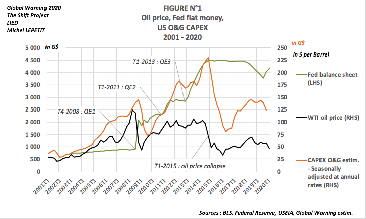
Figure N°2 shows something well-known by macroeconomists; World O&G CAPEX and World oil price series fit nicely on a long-term basis.

The cure to high price is high price AND …

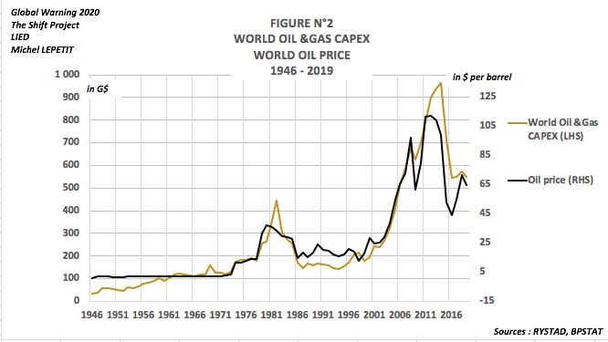
On the long run, the same fit can be seen for oil price and U.S. O&G CAPEX from the 1960s to 2008. But in Figure N°3 (in constant $) the use of oil price as a proxy for the 2010s’ U.S. O&G CAPEX deteriorated. Investments in the Energy industry, especially in the shale oil (LTO) industry, were much higher after the 2008 Great Financial Crisis than one could expect from the price driver alone.[7]

This finding was translated in the second part of the UMPUO V1 formula, taking the impact of Quantitative Easing (i.e. large scale of sovereign and sovereign-backed asset purchases by the Fed) into account, through the growth of the Fed’s Balance sheet.

This modeling can be explained by the very intent of Quantitative Easing, which is to lead investors to reallocate their portfolio to riskier assets (the “portfolio balance” channel)[8]. The primary channel through which QE was set in the 2010s was through the risk premium on the asset purchased. By purchasing low risk and sovereign assets, the Fed reduced the amount of these assets held by the private sector, displacing some investors and reducing the holdings of others.

As one can see in Figure N°4, the proxy UMPUO formula V1 fits quite well the real U.S. O&G CAPEX.

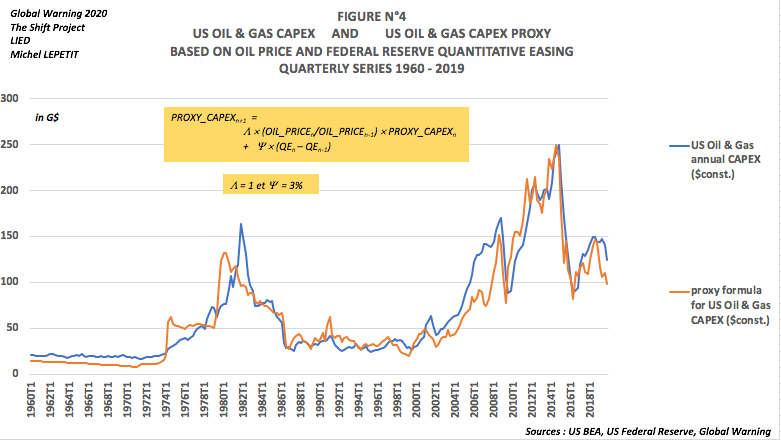
Oil & Gas industry securities, bonds (and loans) were typically the kind of riskier financial assets “portfolio rebalancing” could feed. And it was even riskier for the LTO business which was an innovative segment of the O&G industry, with no track records, and attractive promises.

The huge impact of QE on the U.S. O&G industry – in comparison with other industries – can be explained by the size of the O&G industry in the U.S. prior to 2008. Fundamentally, the O&G industry relies on CAPEX[9]: worldwide, O&G CAPEX is approximately 1/6 of global corporate CAPEX[10]. As most economists know, the cost share of energy, that is its weight in GDP, is low, a fact which does not reflect the major role of energy in the economy. “CAPEX share” of energy is far more substantial than “cost share”[11].

Quantitative Easing of Light Tight Oil (LTO)

Considering that more than $700 Billions of U.S. O&G CAPEX were invested in the shale oil (LTO) industry CAPEX from 2008 to 2019, the – rather simplistic – UMPUO Model V1 would mean that half of this CAPEX, i.e. approximately $350 Billion, could be attributed to Fed Monetary Policy from 2008 to 2019. From a qualitative point of view, this driving role of monetary policy has been pointed out by the Bank of International Settlements (BIS) as soon as 2015 (Domanski 2015)[12].

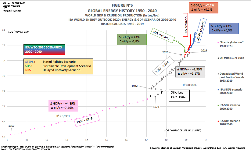
Of course, as said earlier, QE could probably have had a similar impact on other U.S. industry sectors, such as the textile industry through U.S. investments in textile manufacturing assets. But, as many speakers mentioned during the conference, oil is a global key industry. Textile is certainly important, but oil is essential. One could say that oil is the blood of our industrialized civilization. For example, 95% of world transportation and mobility relies on oil. The following graph (Figure N°5)[13] illustrates this strong coupling between oil (in volume)[14] and economic growth. It shows (in Log/log) the intimate link between world GDP and World oil production for the last 70 years (1950-2020), with three IEA scenarios for the next 20 years (2020-2040). Historically, the link between oil (in price) and inflation is so strong, that economists have had to come up with the bizarre concept of “core inflation”[15], i.e. inflation excluding oil price.

Symptom: the U.S. oil macroeconomic puzzle

Many speakers at the conference spoke about the missing “capital discipline”, so widespread in the shale oil industry during the 2010s. The fact is that QE triggered a thirst for risk, which led to a rush in risky projects, too often with low profitability.

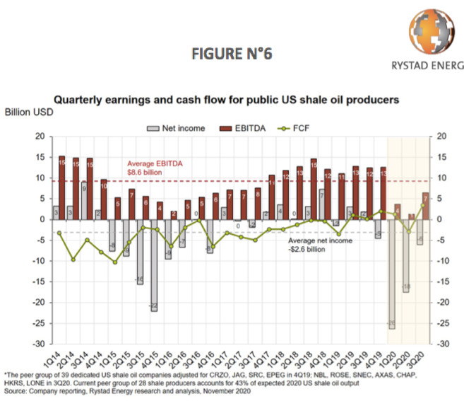
As a matter of fact, one of the major symptoms of the impact of QE on the U.S. oil market risk premium is the non-profitability of the shale oil industry, in globo. As everyone knows, this industry has never been profitable. Rystad reminded of this structural non-profitability again in November 2020[16] using the following graph showing the Free Cash Flow of the shale oil producers (Figure N° 6):

Conclusion: gold, and black gold

In 1970, U.S. conventional crude oil production reached its geophysical apex. It was followed a few months later by a key event in Global World History: on August 15^th, 1971, the U.S. decided to end the convertibility of the U.S. dollar to gold.

In 2006, world conventional crude oil production reached its geophysical apex[17]. It was followed a few month later by another key event in Global World History: on November 25^th, 2008, the Fed inaugurated a global new area of Unconventional Monetary Policy.

The academic paper you refer to, Mrs. George, pretends that high interest rates would increase the supply of commodity (Frankel 2008)[18]. One would say that oil is a very singular commodity. In 2010 the SEC revised its rules for oil reserve accounting[19]. A key SEC concept is “economic producibility of reserves” which, according to the SEC’s definition “must be based on existing economic conditions.” On the long run, from the 1980s to the 2010s, the massive decrease of interest rates down to the zero-lower bound deeply changed the macroeconomic “existing conditions” by rendering “producible” projects that would not have been considered as such a few years earlier. You rightly complemented Frankel’s rather strange statement when you wrote: ”(…) low rates should incentivize investment in the energy sector, and generally, by decreasing the cost of capital.(…)”. Lowering rates certainly incentivized investment in the energy sector, decreasing the cost of capital to levels beyond imagination.

In conclusion, the shale oil revolution has been, by far, the main driver of world crude oil production from 2008 to 2019. Without the U.S. LTO production surge in both Texas and Kansas, world crude oil production would have plateaued in the 2010s. A large part, maybe half, of that tremendous surge of non-profitable oil extraction was a consequence of the American Unconventional Monetary Policy.

Mrs. George, Mr. Kaplan, I think you were right when you said that U.S. Monetary policy was neutral with regard to oil. But, could it be that oil has not been that neutral with regard to monetary policy?

Très cordialement, et encore merci,

Michel LEPETIT

The Shift Project Vice-President

Global Warning CEO

LIED Research Associate

Energy & Prosperity Chair expert

Notes

[1] Initial publication on my LinkedIn profile – I want to thank here all the collaborators and friends at The Shift Project, LIED and ASPO that have provided relevant perspectives to the following research project.

[2] Jens Weidmann – Combating climate change – What central banks can and cannot do – Speech at the European Banking Congress 20/11/2020

(…) Our purchases of private bonds are thus guided by the principle of “market neutrality”. (…) Indeed, studies suggest that the Eurosystem’s corporate bond purchases have compressed yield spreads not only for those bonds purchased or targeted, but also for non-eligible bonds. (…) Such an indirect impact can be due to the portfolio rebalancing channel, as our purchases may push investors into riskier asset classes. Thus, even those “green” bonds that are not eligible might have benefitted from our purchases to some degree. At the same time, the impact of potentially excluding carbon-intensive firms from our portfolio should not be overestimated.(…)

[3] Energy, Economic Activity and Monetary Policy, November 20, 2020
Remarks by Esther L. George, President and CEO, Federal Reserve Bank of Kansas City “

(…) Monetary Policy’s Influence on the Energy Sector

I will close with some thoughts on the influence of monetary policy on the energy sector. To the extent that direct and indirect spillovers affect the economic outlook, and thus monetary policy settings, it is worth considering how monetary policy, and particularly the prospect of low-for-long interest rates, might affect the energy sector. There is a long literature that suggests, all else equal, that low interest rates should boost the price of storable commodities, such as oil, partly by incentivizing greater demand, but also by decreasing the incentive to produce. (11) Converting oil reserves into currency and other assets is less appealing when the return on alternative assets is low. In addition, there is a literature that suggests that low rates should lead to less-volatile prices. Interest rates are an important cost of holding inventory, so low rates should lower inventory costs and incentivize larger buffers that can then mitigate unexpected shifts in supply and demand. (12) Of course there are many other factors affecting oil prices besides interest rates, so low oil prices and continued price volatility can certainly coincide with low-for-long rates.

Again relying on “all else equal,” low rates should incentivize investment in the energy sector, and generally, by decreasing the cost of capital. This could be particularly true in the renewables sector, which has long-lived capital investment with high initial costs similar to utilities more generally. However, low interest rates can work not only by promoting new additions to the capital stock, but also through the acquisition of pre-existing capital—that is by encouraging mergers and acquisitions (M&A). In an industry with uncertain near-term and long-term demand, it might not be surprising to see low rates engender a greater response in M&A activity and consolidation as opposed to increased capital expenditure.”
(11) See Jeffrey Frankel, the Effect of Monetary Policy on Real Commodity Prices, Chapter 7, in Asset prices and Monetary Policy, John Campbell, ed., (U. Chicago Press), 2008 : 291-327
(12) See Gruber, Joseph and Robert Vigfusson “Do Low Interest Rates Decrease Commodity Price Volatility?” IFDP Note 2013-09-26, Board of Governors of the Federal Reserve System, 2013.
[my emphasis]

[4] Global Warning will soon publish an analysis of Federal Reserve regular meetings from 2008 to 2010 (Source: ttps://www.federalreserve.gov/monetarypolicy.htm) focusing on the impact of the Fed monetary policy on shale oil development, oil price and inflation that followed Quantitative Easing Program N°1 in 2008. These are excerpts from minutes of the regular meetings (mostly “beige book” and meeting transcript), preparatory documents (memos) and statements. With particular attention to evolution in the Texas District (Federal Reserve Bank of Dallas), where most of shale oil plays are located.
The key takeaway is that Archives material show that there was no sectoral targeting of the U.S. oil industry by the Federal Board in 2009-2010. The first time U.S. crude oil growth is mentioned is in December 2009. “Light Tight Oil” vocabulary appears late in the transcripts; March 2010. In December 2009 there were many references to Oil Capital Expenditure (CAPEX) boom in some of the Fed regional briefs, and there was the first mention of “shale-based natural gas” in the Dallas District Report. In March 2010 reports, the word “shale” is used four times. Symptoms of overheat in the Oil & Gas sector are obvious at that time; “(…). However, producers in the Kansas City District were concerned that a boost in supply from shale gas production could lower natural gas prices later in the year. (…)”) and April 2010 (“(…). Contacts say the increase in gas-directed drilling is not justifiable at current low prices, but firms are drilling based on futures prices locked in earlier, to hold leases and to learn the shale technology. (…)”).

[5] The quarterly series for O&G CAPEX is an estimation. It is reconstructed from U.S. BEA “Table 5.3.5. Private Fixed Investment by Type” quarterly table: use the “Mining exploration, shafts, and wells” quarterly data series. The quarterly O&G CAPEX is the addition of “O&G Shaft and Well” CAPEX, and “O&G Machinery” CAPEX. O&G Machinery CAPEX is reconstructed from U.S. BEA table “Table 2.1. Current-Cost Net Stock of Private Fixed Assets, Equipment, Structures, and Intellectual Property Products by Type”: use the “Mining and oilfield machinery” yearly data series. The yearly ratio between mining CAPEX and O&G CAPEX (approx. 5%) used in this reconstruction of the quarterly series, is based on U.S. BEA Table 5.4.5. “Private Fixed Investment in Structures by Type”: use the “Petroleum and natural gas” yearly data serie; and the “Mining” yearly data series.

[6] Lepetit Michel, West Slide Story : Unconventional monetary Policy & Unconventional Oil (UMPUO 2000 – 2020), 2020

Scene I – The “Chinese Great Wall” [T1 2001 – T3 2008]
Scene II – The “only game in town” and the shale plays: heavy Quantitative Easing for Light Tight Oil [T4 2008 – T1 2009]
Scene III – The Shaft Project [T2 2009 – T3 2010]
Scene IV – Well Being [T4 2010 – T3 2012]
Scene V – Capital indiscipline [T4 2012 – T3 2014]
Scene VI – Interest rates & oil price are intimately “Low for Long” [T4 2014 – T1 2018
Scene VII – Shale player (over)shoot again [T2 2018 – T4 2019]

[7] As a matter of fact, one can also see this underestimation for world O&G CAPEX in Figure N°2

[8] Federal Reserve, 2015 “What were the Federal Reserve’s large-scale asset purchases?”

“(…) Thus, the overall effect of the Fed’s LSAPs was to put downward pressure on yields of a wide range of longer-term securities, support mortgage markets, and promote a stronger economic recovery.(…)”

[10] See for instance : Global Corporate Capex Survey 2019 – S&P Global Ratings- 19/06/2019

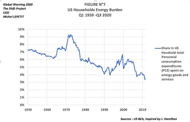
[11] See Lepetit M. (2020a) : Secular Stagnation post COVD-19 & Oil : Just stagnation ? Really ? – 18/03/2020, especially note N° 19 on Larry Summer’s comment on energy cost share. Following J. Hamilton, the following graph shows the energy cost share of US Household PCE.

[12] Domanski Dietrich, Jonathan Kearns, Marco Jacopo Lombardi & Hyun Song Shin – Oil and debt – BIS Quarterly Review – March 2015. https://www.bis.org/publ/qtrpdf/r_qt1503f.htm

“(…) US oil companies have also borrowed heavily. They account for around 40% of both syndicated loans and debt securities outstanding. Much of this debt has been issued by smaller companies, in particular those engaged in shale oil exploration and production. Indeed, while the ratio of total debt to assets has been broadly unchanged for large US oil firms, it has on average almost doubled for other US producers – including smaller shale oil companies. These firms borrowed heavily to finance the expansion of production capacity, often against the backdrop of negative operating cash flow. Indeed, shale investment accounts for a large share of the increase in oil-related investment. Annual capital expenditure by oil and gas companies has more than doubled in real terms since 2000, to almost $900 billion in 2013 (IEA (2014)). (…) The greater willingness of investors to lend against oil reserves and revenue has enabled oil firms to borrow large amounts in a period when debt levels have increased more broadly due to easy monetary policy. Since 2008, companies in the oil sector have borrowed both from banks and in bond markets. Issuance of debt securities by oil and other energy companies has far outpaced the substantial overall issuance by other sectors (Graph 2, left-hand panel). Oil and gas companies’ bonds outstanding increased from $455 billion in 2006 to $1.4 trillion in 2014, a growth rate of 15% per annum. Energy companies have also borrowed heavily from banks. Syndicated loans to the oil and gas sector in 2014 amounted to an estimated $1.6 trillion, an annual increase of 13% from $600 billion in 2006.

Overall, the stock of debt of energy firms has risen even faster than that of other sectors. Debt issued by oil and other energy firms accounts for about 15% of both investment grade and high-yield major US debt indices, up from less than 10% just five years earlier.(…)”

[13] Graph N°5 was inspired by : Hamilton J. (2009) – Causes and Consequences of the Oil Shock of 2007–08 – Brookings Papers on Economic Activity, Spring 2009

[14] As world oil production and consumption are very near figures, we use generally crude oil production. But given the 2020 COVID-19 accident, the figure use for 2020 is consumption. Huge excess inventories will probably not be back to normal at the end of 2020.

[15] See the literature on oil price and its impact on global inflation:

Furceri D. – Global Disinflation in an Era of Constrained Monetary Policy – Furceri Davide & als – IMF WEO 2016 Chapter 3, October 2016
Furceri D. – Oil Prices and Inflation Dynamics: Evidence from Advanced and Developing Economies – Sangyup Choi, Davide Furceri & als – IMF Working Paper 2017
Ha, J, M A Kose, and F Ohnsorge – “Inflation in emerging and developing economies: evolution, drivers and policies.” – World Bank Group 2019

[16] US shale oil producers generated the highest FCF in industry history – Rystad – 19/11/20

[17] IEA WEO 2010

[18] Jeffrey Frankel, the Effect of Monetary Policy on Real Commodity Prices, Chapter 7, in Asset prices and Monetary Policy, John Campbell, ed., (U. Chicago Press), 2008 : 291-327

“(…) Eﬀect of U.S. Short-Term Real Interest Rates on Real U.S. Commodity Prices

The argument can be stated in an intuitive way that might appeal to practitioners as follows. High interest rates reduce the demand for storable commodities, or increase the supply, through a variety of channels: – By increasing the incentive for extraction today rather than tomorrow (think of the rates at which oil is pumped, zinc is mined, forests logged, or livestock herds culled) – By decreasing ﬁrms’ desire to carry inventories (think of oil inventories held in tanks) – By encouraging speculators to shift out of commodity contracts (especially spot contracts) and into treasury bills (…)”

[19] United States – Securities and Exchange Commission. – Modernization of Oil and Gas Reporting Agency – Effective date : 1/01/2010. https://www.sec.gov/rules/final/2008/33-8995.pdf
Note that this SEC amendments were promulgated before the shale oil revolution, its technological fast progress, but its amazing depletion rate of shale oil wells.